标签：training task Learning parameters Meta meta learning Need data

Meta-Learning Is All You Need

2020-06-04 18:57:21

Source：https://medium.com/cracking-the-data-science-interview/meta-learning-is-all-you-need-3bd0bafdf289 

 

Neural networks have been highly influential in the past decades in the machine learning community, thanks to the rise of computing power, the abundance of unstructured data, and the advancement of algorithmic solutions. However, it is still a long way for researchers to completely use neural networks in real-world settings where the data is scarce, and requirements for model accuracy/speed are critical.

Meta-learning, also known as learning how to learn, has recently emerged as a potential learning paradigm that can absorb information from one task and generalize that information to unseen tasks proficiently. During this quarantine time, I started watching lectures on Stanford’s CS 330 class on Deep Multi-Task and Meta-Learning taught by the brilliant Chelsea Finn. As a courtesy of her talks, this blog post attempts to answer these key questions:

1. Why do we need meta-learning?
2. How does the math of meta-learning work?
3. What are the different approaches to design a meta-learning algorithm?

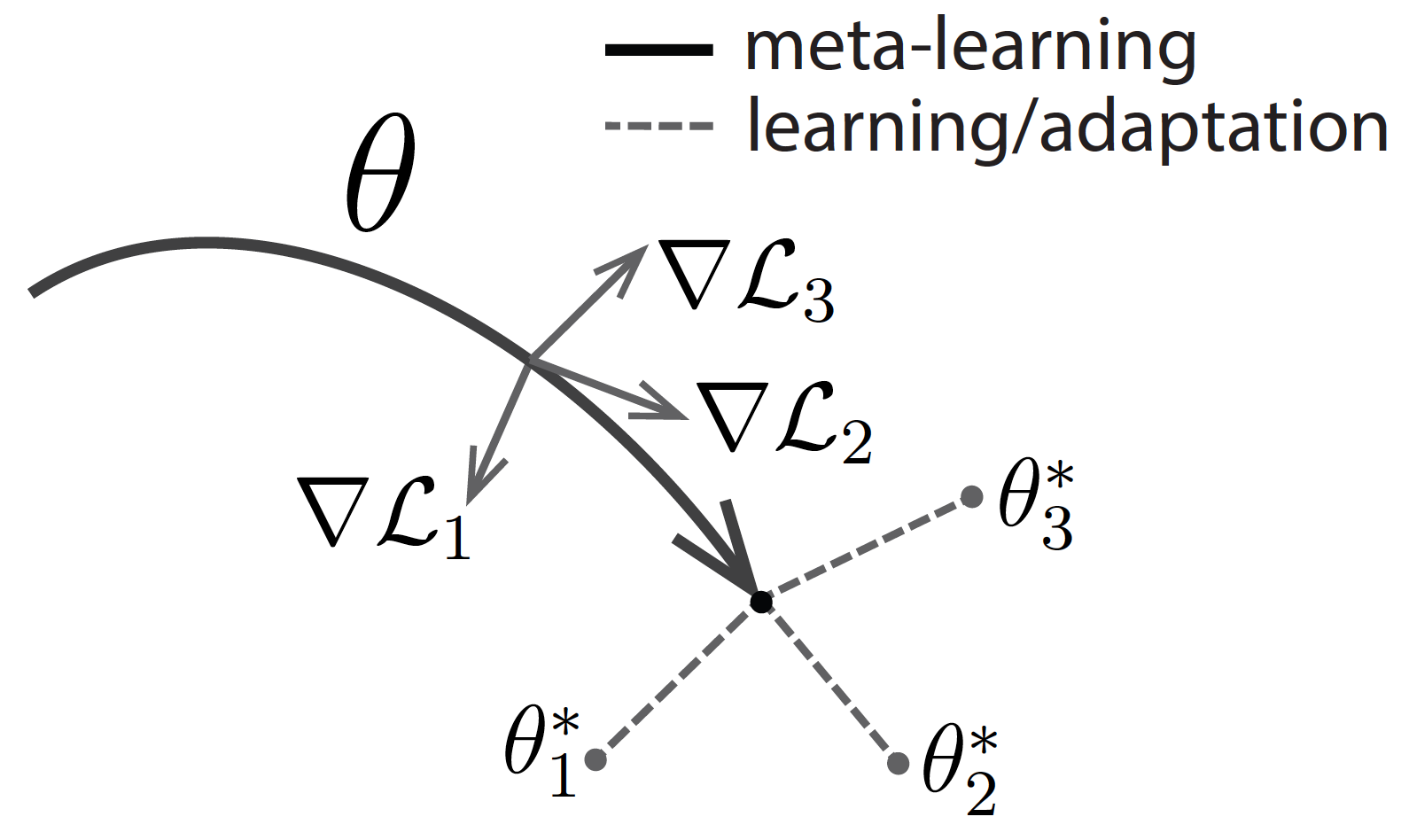  Diagram of Model-Agnostic Meta-Learning — Chelsea Finn in “Learning to Learn”

Note: The content of this post is primarily based on CS330’s lecture one on problem definitions, lecture two on supervised and black-box meta-learning, lecture three on optimization-based meta-learning, and lecture four on few-shot learning via metric learning. They are all accessible to the public.

1 — Motivation For Meta-Learning

Thanks to the advancement in algorithms, data, and compute power in the past decade, deep neural networks have allowed us to handle unstructured data (such as images, text, audio, video, etc.) very well without the need to engineer features by hand. Empirical research has shown that if neural networks can generalize very well if we feed them large and diverse inputs. For example, Transformers and GPT-2 made the wave in the Natural Language Processing research community last year with their broad applicability in various tasks.

However, there is a catch with using neural networks in the real-world setting where:

• Large datasets are unavailable: This issue is common in many domains ranging from classification of rare diseases to translation of uncommon languages. It is impractical to learn from scratch for each task in these scenarios.
• Data has a long tail: This issue can easily break the standard machine learning paradigm. For example, in the self-driving car setting, an autonomous vehicle can be trained to handle everyday situations very well. Still, it often struggles with uncommon conditions (such as people jay-walking, animal crossing, traffic lines not working) where humans can comfortably handle. This can lead to awful outcomes, such as the Uber’s accident in Arizona a few years ago.
• We want to quickly learn something about a new task without training our model from scratch: Humans can do this quite easily by leveraging our prior experience. For example, if I know a bit of Spanish, then it should not be too difficult for me to learn Italian, as these two languages are quite similar linguistically.

In this article, I would like to give an introductory overview of meta-learning, which is a learning framework that can help our neural network become more effective in the settings mentioned above. In this setup, we want our system to learn a new task more proficiently — assuming that it is given access to data on previous tasks.

Historically, there have been a few papers thinking in this direction.

• Back in 1992, Bengio et al. looked at the possibility of a learning rule that can solve new tasks.
• In 1997, Rich Caruana wrote a survey about multi-task learning, which is a variant of meta-learning. He explained how tasks could be learned in parallel using a shared representation between models and also presented a multi-task inductive transfer notion that uses back-propagation to handle additional tasks.
• In 1998, Sebastian Thrun explored the problem of lifelong learning, which is inspired by the ability of humans to exploit experiences that come from related learning tasks to generalize to new tasks.

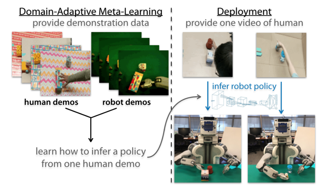  Figure 1: The Domain-Adaptive Meta-Learning system described in Yu et al.

Right now is an exciting period to study meta-learning because it is increasingly becoming more fundamental in machine learning research. Many recent works have leveraged meta-learning algorithms (and their variants) to do well for the given tasks. A few examples include:

• Aharoni et al. expand the number of languages used in a multi-lingual neural machine translation setting from 2 to 102. Their method learns a small number of languages and generalizes them to a vast amount of others.
• Yu et al. present Domain-Adaptive Meta-Learning (figure 1), a system that allows robots to learn from a single video of a human via prior meta-training data collected from related tasks.
• A recent paper from YouTube shows how their team used multi-task methods to make video recommendations and handle multiple competing ranking objectives.

Forward-looking, the development of meta-learning algorithms will help democratize deep learning and solve problems in domains with limited data.

2 — Basics of Meta-Learning

In this section, I will cover the basics of meta-learning. Let’s start with the mathematical formulation of supervised meta-learning.

2.1 — Formulation

In a standard supervised learning, we want to maximize the likelihood of model parameters ϕ given the training data D:

  Equation 1

Equation 1 can be redefined as maximizing the probability of the data provided the parameters and maximizing the marginal probability of the parameters, where p(D|ϕ) corresponds to the data likelihood, and p(ϕ) corresponds to a regularizer term:

  Equation 2

Equation 2 can be further broken down as follows, assuming that the data D consists of (input, label) pairs of (xᵢ, yᵢ):

  Equation 3

However, if we deal with massive data D (as in most cases with complicated problems), our model will likely overfit. Even if we have a regularizer term here, it might not be enough to prevent that from happening.

The critical problem that supervised meta-learning solves is: Is it feasible to get more data when dealing with supervised learning problems?

  Figure 2: The Meta-Learning setup described in “Optimization as a Model for Few-Shot Learning.”

Ravi and Larochelle’s “Optimization as a Model for Few-Shot Learning” is the first paper that provides a standard formulation of the meta-learning setup, as seen in figure 2. They reframe equation 1 to equation 4 below, where D_{meta-train} is the meta-training data that allows our model to learn more efficiently. Here, D_{meta-train} corresponds to a set of datasets for predefined tasks D₁, D₂, …, Dn:

Next, they design a set of meta-parameters θ = p(θ|D_{meta-train}), which includes the necessary information about D_{meta-train} to solve the new tasks.

  Equation 4

Mathematically speaking, with the introduction of this intermediary variable θ, the full likelihood of parameters for the original data given the meta-training data (in equation 4) can be expressed as an integral over the meta-parameters θ:

  Equation 5

Equation 5 can be approximated further with a point estimate for our parameters:

  Equation 6

• p(ϕ|D, θ*) is the adaptation task that collects task-specific parameters ϕ or a new task — assuming that it has access to the data from that tas D and meta-parameters θ.
• p(θ* | D_{meta-train}) is the meta-training task that collects meta-parameters θ — assuming that it has access to the meta-training data D_{meta-train}).

To sum it up, the meta-learning paradigm can be broken down into two phases:

• The adaptation phase: ϕ* = arg max log p(ϕ|D,θ*) (first term in equation 6)
• The meta-training phase: θ* = max log p(θ|D_{meta-train}) (second term in equation 6)

2.2 — Loss Optimization

Let’s look at the optimization of the meta-learning method. Initially, our meta-training data consists of pairs of training-test set for every task:

  Equation 7

There are k feature-label pairs (x, y) in the training set Dᵢᵗʳ and l feature pairs (x, y) in the test set Dᵢᵗˢ:

  Equation 8

During the adaptation phase, we infer a set of task-specific parameters ϕ*, which is a function that takes as input the training set Dᵗʳ and returns as output the task-specific parameters: ϕ* = f_{θ*} (Dᵗʳ). Essentially, we want to learn a set of meta-parameters θ such that the function ϕᵢ = f_{θ} (Dᵢᵗʳ) is good enough for the test set Dᵢᵗˢ.

During the meta-learning phase, to get the meta-parameters θ*, we want to maximize the probability of the task-specific parameters ϕ being effective at new data points in the test set Dᵢᵗˢ.

  Equation 9

2.3 — Meta-Learning Paradigm

According to Chelsea Finn, there are two views of the meta-learning problem: a deterministic view and a probabilistic view.

The deterministic view is straightforward: we take as input a training data set Dᵗʳ, a test data point x_test, and the meta-parameters θ to produce the label corresponding to that test input y_test. The way we learn this function is via the D_{meta-train}, as discussed earlier.

  Equation 10

The probabilistic view incorporates Bayesian inference: we perform a maximum likelihood inference over the task-specific parameters ϕᵢ — assuming that we have the training dataset Dᵢᵗʳ and a set of meta-parameters θ:

  Equation 11

Regardless of the view, there two steps to design a meta-learning algorithm:

• Step 1 is to create the function p(ϕᵢ|Dᵢᵗʳ, θ) during the adaptation phase.
• Step 2 is to optimize θ concerning D_{meta-train} during the meta-training phase.

In this post, I will only pay attention to the deterministic view of meta-learning. In the remaining sections, I focus on the three different approaches to build up the meta-learning algorithm: (1) The black-box approach, (2) The optimization-based approach, and (3) The non-parametric approach. More specifically, I will go over their formulation, architectures used, and challenges associated with each method.

3 — Black-Box Meta-Learning

3.1 — Formulation

The black-box meta-learning approach uses neural network architecture to generate the distribution p(ϕᵢ|Dᵢᵗʳ, θ).

• Our task-specific parameters are: ϕᵢ = f_{θ}(Dᵢᵗʳ).
• A neural network with meta-parameters θ (denoted as f_{θ}) takes in the training data Dᵢᵗʳ s input and returns the task-specific parameters ϕᵢ as output.
• Another neural network (denoted as g(ϕᵢ)) takes in the task-specific parameters ϕᵢ as input and returns the predictions about test data points Dᵢᵗˢ as output.

During optimization, we maximize the log-likelihood of the outputs from g(ϕᵢ) for all the test data points. This is applied across all the tasks in the meta-training set:

  Equation 12

The log-likelihood of g(ϕᵢ) in equation 12 is essentially the loss between a set of task-specific parameters ϕᵢ and a test data point Dᵢᵗˢ:

  Equation 13

Then in equation 12, we optimize the loss between the function f_θ(Dᵢᵗʳ) and the evaluation on the test set Dᵢᵗˢ:

  Equation 14

This is the black-box meta-learning algorithm in a nutshell:

• We sample a task T_i, as well as the training set Dᵢᵗʳ and test set Dᵢᵗˢ from the task dataset D_i.
• We compute the task-specific parameters ϕᵢ given the training set Dᵢᵗʳ: ϕᵢ ← f_{θ} (Dᵢᵗʳ).
• Then, we update the meta-parameters θ using the gradient of the objective with respect to the loss function between the computed task-specific parameters ϕᵢ and Dᵢᵗˢ: ∇_{θ} L(ϕᵢ, Dᵢᵗˢ).
• This process is repeated iteratively with gradient descent optimizers.

3.2 — Challenges

The main challenge with this black-box approach occurs when ϕᵢ happens to be massive. If ϕᵢ is a set of all the parameters in a very deep neural network, then it is not scalable to output ϕᵢ.

“One-Shot Learning with Memory Augmented Neural Networks” and “A Simple Neural Attentive Meta-Learner” are two research papers that tackle this. Instead of having a neural network that outputs all of the parameters ϕᵢ, they output a low-dimensional vector hᵢ, which is then used alongside meta-parameters θ to make predictions. The new task-specific parameters ϕᵢ has the form: ϕᵢ = {hᵢ, θ}, where θ represents all of the parameters other than h.

Overall, the general form of this black-box approach is as follows:

  Equation 15

Here, yᵗˢ corresponds to the labels of test data, xᵗˢ corresponds to the features of test data, and Dᵢᵗʳ corresponds to pairs of training data.

3.3 — Architectures

So what are the different model architectures to represent this function f?

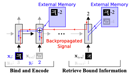  Figure 3 — The memory-augmented neural network as described in “One-Shot Learning with Memory Augmented Neural Networks.”

• Memory Augmented Neural Networks by Santoro et al. uses Long Short-Term Memory and Neural Turing Machine architectures to represent f. Both architectures have an external memory mechanism to store information from the training data point and then access that information during inference in a differentiable way, as seen in figure 3.
• Conditional Neural Processes by Garnelo et al. represents f via 3 steps: (1) using a feed-forward neural network to compute the training data information, (2) aggregating that information, and (3) passing that information to another feed-forward network for inference.
• Meta Networks by Munkhdalai and Yu uses other external memory mechanisms with slow and fast weights that are inspired by neuroscience to represent f. Specifically, the slow weights are designed for meta-parameters θ and the fast weights are designed for task-specific parameters ϕ.

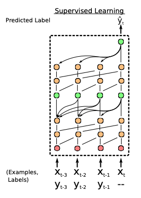  Figure 4: The simple neural attentive meta-learner as described in “A Simple Neural Attentive Meta-Learner.”

• Neural Attentive Meta-Learner by Mishra et al. uses an attention mechanism to represent f. Such a mechanism allows the network to pick out the most important information that it gathers, thus making the optimization process much more efficient, as seen in figure 4.

In conclusion, black-box meta-learning approach has high learning capacity. Given that neural networks are universal function approximators, the black-box meta-learning algorithm can represent any function of our training data. However, as neural networks are fairly complex and the learning process usually happens from scratch, the black-box approach usually requires a large amount of training data and a large number of tasks in order to perform well.

4 — Optimization-Based Meta-Learning

Okay, so how else can we represent the distribution p(ϕᵢ|Dᵢᵗʳ, θ) in the adaptation phase of meta-learning? If we want to infer all the parameters of our network, we can treat this as an optimization procedure. The key idea behind optimization-based meta-learning is that we can optimize the process of getting the task-specific parameters ϕᵢ so that we will get a good performance on the test set.

4.1 — Formulation

Recall that the meta-learning problem can be broken down into two terms below, one that maximizes the likelihood of training data given the task-specific parameters and one that maximizes the likelihood of task-specific parameters given meta-parameters:

  Equation 16

Here the meta-parameters θ are pre-trained during training time and fine-tuned during test time. The equation below is a typical optimization procedure via gradient descent, where α is the learning rate.

  Equation 17

To get the pre-trained parameters, we can use standard benchmark datasets such as ImageNet for computer vision, Wikipedia Text Corpus for language processing, or any other large and diverse datasets that we have access to. As expected, this approach becomes less effective with a small amount of training data.

Model-Agnostic Meta-Learning (MAML) from Finn et al. is an algorithm that addresses this exact problem. Taking the optimization procedure in equation 17, it adjusts the loss so that only the best-performing task-specific parameters ϕ on test data points are considered. This happens for all the tasks:

  Equation 18

The key idea is to learn θ for all the assigned tasks in order for θ to transfer effectively via the optimization procedure.

This is the optimization-based meta-learning algorithm in a nutshell:

• We sample a task Tᵢ, as well as the training set Dᵢᵗʳ and test set Dᵢᵗˢ from the task dataset Dᵢ.
• We compute the task-specific parameters ϕᵢ given the training set Dᵢᵗʳ using the optimization procedure described above: ϕᵢ ← θ — α ∇_θ L(θ, Dᵢᵗʳ)
• Then, we update the meta-parameters θ using the gradient of the objective with respect to the loss function between the computed task-specific parameters ϕᵢ and Dᵢᵗˢ: ∇_{θ} L(ϕᵢ, Dᵢᵗˢ).
• This process is repeated iteratively with gradient descent optimizers.

As provided in the previous section, the black-box meta-learning approach has the general form: yᵗˢ = f_{θ} (Dᵢᵗʳ, xᵗˢ). The optimization-based MAML method described above has a similar form below, where ϕᵢ = θ — α ∇_{θ} L(ϕ, Dᵢᵗʳ):

  Equation 19

To prove the effectiveness of the MAML algorithm, in Meta-Learning and Universality, Finn and Levine show that the MAML algorithm can approximate any function of Dᵢᵗʳ, xᵗˢ for a very deep function f. This finding demonstrates that the optimization-based MAML algorithm is as expressive as any other black-box algorithms mentioned previously.

4.2 — Architectures

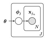  Figure 5: The probabilistic graphical model for which MAML provides an inference procedure as described in “Recasting Gradient-Based Meta-Learning as Hierarchical Bayes.”

In “Recasting Gradient-Based Meta-Learning as Hierarchical Bayes”, Grant et al. provide another MAML formulation as a method for probabilistic inference via hierarchical Bayes. Let’s say we have a graphical model as illustrated in figure 5, where J is the task, x_{j_n} is a data point in that task, ϕⱼ are the task-specific parameters, and θ is the meta-parameters.

To do inference with respect to this graphical model, we want to maximize the likelihood of the data given the meta-parameters:

  Equation 20

The probability of the data given the meta-parameters can be expanded into the probability of the data given the task-specific parameters and the probability of the task-specific parameters given the meta-parameters. Thus, equation 20 can be rewritten as:

  Equation 21

This integral in equation 21 can be approximated with a Maximum a Posteriori estimate for ϕⱼ:

  Equation 22

In order to compute this Maximum a Posteriori estimate, the paper performs inference on Maximum a Posteriori under an implicit Gaussian prior — with mean that is determined by the initial parameters and variance that is determined by the number of gradient steps and the step size.

There have been other attempts to compute the Maximum a Posteriori estimate in equation 22:

• Rajeswaran et al. propose an implicit MAML algorithm that uses gradient descent with an explicit Gaussian prior. More specifically, they regularize the inner optimization of the algorithm to be close to the meta-parameters θ: ϕ ← min_{ϕ’} L(ϕ’, Dᵗʳ) + λ/2 ||θ — ϕ’||². The mean and the variance of this explicit Gaussian prior is a function of λ regularizer.

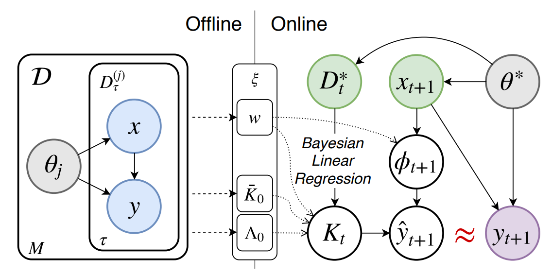  Figure 6: The ALPaCA algorithm which uses Bayesian linear regression as described in “Meta-Learning Priors for Efficient Online Bayesian Regression.”

• Harrison et al. propose the ALPaCA algorithm that uses an efficient Bayesian linear regression on top of the learned features from the inner optimization loop to represent the mean and variance of that regression as meta-parameters themselves (illustrated in figure 6). The inclusion of prior information here reduces computational complexity and adds more confidence to the final predictions.
• Bertinetto et al. attempt to solve meta-learning with differentiable closed-form solutions. In particular, they apply a ridge regression as a base learner for the features in the inner optimization loop. The mean and variance predictions from the ridge regression are then used as meta-parameters in the outer optimization loop.

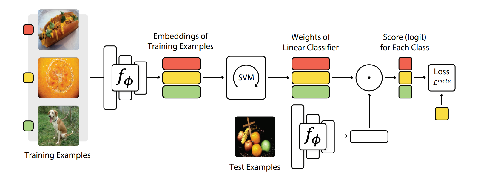  Figure 7: The MetaOptNet approach as described in “Meta-Learning with Differentiable Convex Optimization.”

• Lee et al. attempt to solve meta-learning with differentiable convex optimization solutions. The proposed method, called MetaOptNet, uses a support vector machine to learn the features from the inner optimization loop (as seen in figure 7).

4.3 — Challenges

The MAML method requires very deep neural architecture in order to effectively get a good inner gradient update. Therefore, the first challenge lies in choosing that architecture. Kim et al. propose Auto-Meta, which searches for the MAML architecture. They found that the highly non-standard architectures with deep and narrow layers tend to perform very well.

The second challenge that comes up lies in the unreliability of the two-degree optimization paradigm. There are many different optimization tricks that can be useful in this scenario:

• Li et al. propose Meta-SGD that learns the initialization parameters, the direction of the gradient updates, and the value of the inner learning rate in an end-to-end fashion. This method has proven to increase speed and accuracy of the meta-learner.
• Behl et al. come up with Alpha-MAML, which is an extension of the vanilla MAML. Alpha-MAML uses an online hyper-parameter adaptation scheme to automatically tune the learning rate, making the training process more robust.

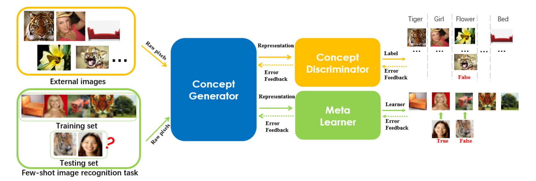  Figure 8: The Deep Meta Learning as described in “Deep Meta-Learning: Learning to Learn in the Concept Space.”

• Zhou et al. devise Deep Meta-Learning, which performs meta-learning in a concept space. As illustrated in figure 8, the concept generator generates the concept-level features from the inputs, while the concept discriminator distinguishes the features generated from that first step. The final loss function includes both the loss from the discriminator and the loss from the meta-learner.
• Zintgraf et al. design CAVIA, which stands for fast context adaptation via meta-learning. To handle the overfitting challenge with vanilla MAML, CAVIA optimizes only a subset of the input parameters in the inner loop at test time (deemed context parameters), instead of the whole neural network. By separating the task-specific parameters and task-independent parameters, they show that training CAVIA is highly efficient.
• Antoniou et al. ideate MAML++, which is a comprehensive guideline on reducing the hyper-parameter sensitivity, lowering the generalization error, and improving MAML stability. One interesting idea is that they disentangle both the learning rate and the batch-norm statistics per step of the inner loop.

In conclusion, optimization-based meta-learning works by constructing a two-degree optimization procedure, where the inner optimization computes the task-specific parameters ϕ and the outer optimization computes the meta-parameters θ. The most representative method is the Model-Agnostic Meta-Learning algorithm, which has been studied and improved upon extensively since its conception.

The big benefit of MAML is that we can optimize the model’s initialization scheme, in contrast to the black box approach where the initial optimization procedure is not optimized. Furthermore, MAML is highly consistent, which extrapolates well to learning problems where the data is out-of-distribution (compared to what the model has seen during meta-training). Unfortunately, because optimization-based meta-learning requires second-order optimization, it is very computationally expensive.

5 — Non-Parametric Meta-Learning

So can we perform the learning procedure described above without a second-order optimization? This is where non-parametric methods fit in.

Non-parametric methods are very effective at learning with a small amount of data (k-Nearest Neighbor, decision trees, support vector machines). In non-parametric meta-learning, we compare the test data with the training data using some sort of similarity metric. If we find the training data that are most similar to the test data, we assign the labels of those training data as the label of the test data.

5.1 — Formulation

This is the non-parametric meta-learning algorithm in a nutshell:

• We sample a task Tᵢ, as well as the training set Dᵢᵗʳ and test set Dᵢᵗˢ from the task dataset Dᵢ.
• We predict the test label yᵗˢ via the similarity between training data and test data (represented by f_θ: yᵗˢ = ∑{x_k, y_k ∈ Dᵗʳ} f_θ (xᵗˢ, x_k) y_k.
• Then we update the meta-parameters θ of this learned embedding function with respect to the loss function of how accurate our predictions are on the test set: ∇_{θ} L(yᵗˢ, yᵗˢ).
• This process is repeated iteratively with gradient descent optimizers.

Unlike the black-box and optimization-based approaches, we no longer have the task-specific parameters ϕ, which is not required for the comparison between training and test data.

5.2 — Architectures

Now let’s go over the different architectures used in non-parametric meta-learning methods.

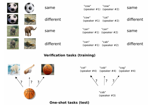  Figure 9: The Siamese Network strategy devised in “Siamese Neural Network for One-Shot Image Recognition.”

Koch et al. propose a Siamese network that consists of two tasks: the verification task and the one-shot task. Taking in pairs of images during training time, the network verifies whether they are of the same class or different classes. At test time, the network performs one-shot learning: comparing each image xᵗˢ to the images in the training set Dⱼᵗʳ for a respective task and predicting the label of xᵗˢ that corresponds to the label of the closest image. Figure 9 illustrates this strategy.

Vinyals et al. propose Matching Networks, which matches the actions happening during training time at test time. The network takes the training data and the test data and embeds them into their respective embedding spaces. Then, the network compares each pair of train-test embeddings to make the final label predictions:

  Equation 23 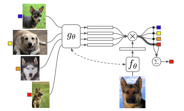  Figure 10: The Matching Networks architecture described in “Matching Networks for One-Shot Learning.”

The Matching Network architecture used in Matching Networks includes a convolutional encoder network to embed the images and a bi-directional Long-Short Term Memory network to produce the embeddings of such images. As seen in figure 10, the examples in the training set match the examples in the test set.

Snell et al. propose Prototypical Networks, which create prototypical embeddings for all the classes in the given data. Then, the network compares those embeddings to make the final label predictions for the corresponding class.

Figure 11 provides a concrete illustration of how Prototypical Networks look like in the few-shot scenario. c₁, c₂, and c₃ are the class prototypical embeddings, which are computed as:

  Equation 24 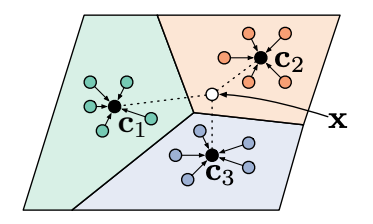  Figure 11: Prototypical Networks as described in “Prototypical Networks for Few-Shot Learning.”

Then, we compute the distances from x to each of the prototypical class embeddings: D(fθ(x), c_k).

To get the final class prediction p_θ(y=k|x), we look at the probability of the negative distances after a softmax activation function, as seen below:

  Equation 25

5.3 — Challenge

For non-parametric meta-learning, how can we learn deeper interactions between our inputs? The nearest neighbor probably will not work well when our data is high-dimensional. Here are three papers that attempt to accomplish this:

• Sung et al. come up with RelationNet (figure 12), which has two modules: the embedding module and the relation module. The embedding module embeds the training and test inputs to training and test embeddings. Then the relation module takes in the embeddings and learns a deep distance metric to compare those embeddings (function D in equation 25).
• Allen et al. propose an Infinite Mixture of Prototypes. This is an extension of the Prototypical Networks, in the sense that it adaptively sets the model capacity based on the data complexity. By assigning each class its own cluster, this method allows the use of unsupervised clustering, which is helpful for many purposes.
• Garcia and Bruna use a Graph Neural Network in their meta-learning paradigm. By mapping the inputs into their graphical representation, they can easily learn the similarity between training and test data via the edge and node features.

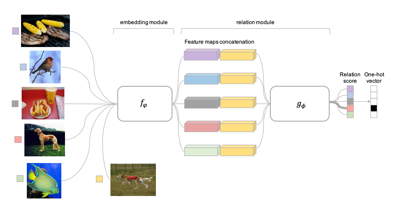  Figure 12: Relation Networks as described in “Learning to Compare: Relation Network for Few-Shot Learning.”

6 — Conclusion

In this post, I have discussed the motivation for meta-learning, the basic formulation and optimization objective for meta-learning, as well as the three approaches regarding the design of the meta-learning algorithm. In particular:

• Black-box meta-learning algorithms have very strong learning capacity, in the sense that neural networks are universal function approximators. But if we impose certain structures into the function, there is no guarantee that black-box models will produce consistent results. Additionally, we can use black-box approaches with different types of problem settings such as reinforcement learning and self-supervised learning. However, because black-box models always learn from scratch, they are very data-hungry.
• Optimization-based meta-learning algorithms can be reduced down to gradient descent; thus, it’s reasonable to expect consistent predictions. For deep enough neural networks, optimization-based models also have very high capacity. Because the initialization is optimized internally, optimization-based models have a better head-start than black-box models. Furthermore, we can try out different architectures without any real difficulty, as evidenced by the Model-Agnostic Meta-Learning (MAML) learning paradigm. However, the second-order optimization procedure makes optimization-based approaches quite computationally expensive.
• Non-parametric meta-learning algorithms have good learning capacity for most choices of architectures as well as good learning consistency under the assumption that the learned embedding space is effective enough. Furthermore, non-parametric approaches do not involve any back-propagation, so they are computationally fast and easy to optimize. The downside is that they are hard to scale to large batches of data because they are non-parametric.

There are a lot of exciting directions for the field of meta-learning, such as Bayesian Meta-Learning (the probabilistic view of meta-learning) and Meta Reinforcement Learning (the use of meta-learning in the reinforcement learning setting). I’d certainly expect to see more real-world applications in wide-ranging domains such as healthcare and manufacturing using meta-learning under the hood. I’d highly recommend going through the course lectures and take detailed notes on the research on these topics!

This post is originally published on my website!

---

If you would like to follow my work on Recommendation Systems, Deep Learning, MLOps, and Data Journalism, you can follow my Medium and GitHub, as well as other projects at https://jameskle.com/. You can also tweet at me on Twitter, email me directly, or find me on LinkedIn. Or join my mailing list to receive my latest thoughts right at your inbox!

标签：training,task,Learning,parameters,Meta,meta,learning,Need,data
来源： https://www.cnblogs.com/wangxiaocvpr/p/13045472.html

本站声明： 1. iCode9 技术分享网（下文简称本站）提供的所有内容，仅供技术学习、探讨和分享；
2. 关于本站的所有留言、评论、转载及引用，纯属内容发起人的个人观点，与本站观点和立场无关；
3. 关于本站的所有言论和文字，纯属内容发起人的个人观点，与本站观点和立场无关；
4. 本站文章均是网友提供，不完全保证技术分享内容的完整性、准确性、时效性、风险性和版权归属；如您发现该文章侵犯了您的权益，可联系我们第一时间进行删除；
5. 本站为非盈利性的个人网站，所有内容不会用来进行牟利，也不会利用任何形式的广告来间接获益，纯粹是为了广大技术爱好者提供技术内容和技术思想的分享性交流网站。