标签:loss 01 nn self torch 学习 Pytorch 深入 size
Pytorch学习二阶段
一、自动求导
训练神经网络包含两步:
- 前向传播
- 后向传播:后向传播中,NN将调整他的参数,并通过loss_function来自计算误差,并通过优化器来优化参数。
import torch, torchvision
model = torchvision.models.resnet18(pretrained=True)
data = torch.rand(1, 3, 64, 64)
labels = torch.rand(1, 1000)

prediction = model(data) # forward pass

>>>data
tensor([[[[0.0792, 0.3683, 0.3258,  ..., 0.8572, 0.9326, 0.5032],
          [0.3238, 0.3992, 0.6769,  ..., 0.7879, 0.6261, 0.4239],
          [0.0839, 0.7466, 0.7469,  ..., 0.0616, 0.5267, 0.0221],
          ...,
          [0.4114, 0.2793, 0.4946,  ..., 0.3337, 0.0151, 0.9790],
          [0.4874, 0.2718, 0.3890,  ..., 0.6204, 0.2941, 0.9589],
          [0.8202, 0.3904, 0.9375,  ..., 0.1282, 0.2416, 0.0420]],

         [[0.2958, 0.6416, 0.2069,  ..., 0.0054, 0.3710, 0.8716],
          [0.2861, 0.6640, 0.3595,  ..., 0.4552, 0.6691, 0.9000],
          [0.1908, 0.1988, 0.0502,  ..., 0.9516, 0.0986, 0.2951],
          ...,
          [0.3542, 0.6152, 0.8829,  ..., 0.7102, 0.7418, 0.2471],
          [0.1259, 0.4121, 0.4195,  ..., 0.0277, 0.7919, 0.1961],
          [0.6761, 0.1635, 0.6317,  ..., 0.5082, 0.8117, 0.4959]],...
>>>labels
tensor([[9.7649e-01, 7.4230e-01, 8.9876e-01, 3.9301e-01, 4.3104e-01, 2.5916e-01,
         2.1638e-01, 2.3715e-01, 3.6239e-01, 5.1230e-02, 5.0033e-01, 9.3420e-01,
         7.3738e-01, 5.1232e-01, 6.1602e-01, 3.1946e-01, 3.3043e-01, 6.6394e-01,
         6.5134e-01, 4.4163e-01, 3.2559e-01, 1.1167e-01, 9.5033e-01, 2.6302e-01,
         4.9590e-01, 1.1047e-01, 6.7810e-01, 1.6822e-01, 3.9666e-01, 9.3511e-01,...
计算完毕前向传播后,通过与真实标签计算误差(目前常用交叉熵去计算)。然后下一步就是后向传播误差在网络参数中,自动梯度计算并存储了梯度为每个参数,通过.grad属性。
loss = (prediction - labels).sum()
loss.backward() # backward pass

>>> loss
tensor(-491.3782, grad_fn=<SumBackward0>)
接下来定义优化器,用随机梯度下降,SGD,并且Learning_rate设置为0.01,动量设置为0.9。
optim = torch.optim.SGD(model.parameters(), lr=1e-2, momentum=0.9)

>>> optim
SGD (
Parameter Group 0
    dampening: 0
    lr: 0.01
    momentum: 0.9
    nesterov: False
    weight_decay: 0
)
最后我们调用.step()来初始玩成梯度下降,优化器最后会调整参数通过模型属性.grad。
optim.step() #gradient descent
(一)Autograd中的分化
autograd是怎样收集梯度的呢?
举例如下:
import torch

a = torch.tensor([2., 3.], requires_grad=True)
b = torch.tensor([6., 4.], requires_grad=True)
假设a,b都是NN的参数,Q是损失,在训练过程,优化参数求导:
\[\frac{∂Q}{∂a}=9a^2 \]\[\frac{∂Q}{∂b}=-2b \]当调用.backward()在Q上,autograd计算这些梯度和分数,在参数的.grad属性。

在idea中可以看到,未学习前,grad为0空,下图是autograd计算后,得到的a的值,b同理可得。

(二)向量计算使用autograd
在数学里,雅各比行列式被用来存储函数的导数:

而autograd也可以用来计算雅各比行列式。
(三)计算图
计算图是autograd的一种计算方法,称之为directed acyclic graph,在DAG中,叶子是输入张量,根是输出张量,通过追踪计算图的叶子到根,我们可以自动计算出梯度,使用链式法则。
前向传播中,autograd同时做两件事情:
- 运行必要的计算操作
- 保持梯度函数的操作,在DAG中
后向传播当.backward()被调用在DAG的根上,autograd则:
- 计算梯度的每个
.grad_fn - 加快张量的
.grad属性计算 - 使用链式法则,传播给所连的叶子张量
DAG记录了每个张量的操作,当其requires_grad标志位设置为True,反之,将不会记录。在NN中,参数不更新叫做冻结参数(frozen parameters),如果你事先直到不需要梯度更新参数,这将是有用的。
from torch import nn, optim

model = torchvision.models.resnet18(pretrained=True)

# Freeze all the parameters in the network
for param in model.parameters():
    param.requires_grad = False
二、NEURAL NETWORKS
一个典型的神经网络训练过程:
- 定义NN(一些可以学习的参数)
- 迭代输入的数据集
- 计算损失
- 运用后向传播和梯度
- 更新权重,一般简单的运用公式:
weight = weight - learning_rate * gradient
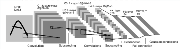
(一)定义网络
class Net(nn.Module):

    def __init__(self):
        super(Net, self).__init__()
        # 1 input image channel, 6 output channels, 5x5 square convolution
        # kernel
        self.conv1 = nn.Conv2d(1, 6, 5)
        self.conv2 = nn.Conv2d(6, 16, 5)
        # an affine operation: y = Wx + b
        self.fc1 = nn.Linear(16 * 5 * 5, 120)  # 5*5 from image dimension
        self.fc2 = nn.Linear(120, 84)
        self.fc3 = nn.Linear(84, 10)

    def forward(self, x):
        # Max pooling over a (2, 2) window
        x = F.max_pool2d(F.relu(self.conv1(x)), (2, 2))
        # If the size is a square, you can specify with a single number
        x = F.max_pool2d(F.relu(self.conv2(x)), 2)
        x = torch.flatten(x, 1) # flatten all dimensions except the batch dimension
        x = F.relu(self.fc1(x))
        x = F.relu(self.fc2(x))
        x = self.fc3(x)
        return x


net = Net()
print(net)

>>>Net(
  (conv1): Conv2d(1, 6, kernel_size=(5, 5), stride=(1, 1))
  (conv2): Conv2d(6, 16, kernel_size=(5, 5), stride=(1, 1))
  (fc1): Linear(in_features=400, out_features=120, bias=True)
  (fc2): Linear(in_features=120, out_features=84, bias=True)
  (fc3): Linear(in_features=84, out_features=10, bias=True)
)
forward必须被定义,但是backward函数不需要,因为已经被自动定义。forward可以被用于任何张量操作。
Note:
torch.nn仅支持mini-batches。nn.Conv2d将喂入一个4dimension的张量,如nSamples x nChannels x Height x Width。如果是一个单个样本,使用input.unsqueeze(0)去增加一个虚拟batch维度。
Recap:
-
torch.Tensor是一个多维向量,支持autograd -
nn.Moduleneural network模型,转化参数类型,可以移步到GPU去计算 -
nn.Parameter一种张量,可以自动地注册 -
autograd.Function实现了autograd操作的前后传播定义,每一个张量操作创造至少一个Function节点,以此链接特殊的函数,这个特殊的函数创建了一个张量,并且编码了它的生命记录
(二)损失函数
损失函数需要输出和目标值作为一对输入,并且计算他们俩之间的差距。
output = net(input)
target = torch.randn(10)  # a dummy target, for example
target = target.view(1, -1)  # make it the same shape as output
criterion = nn.MSELoss()

loss = criterion(output, target)
print(loss)

>>>
tensor(0.6493, grad_fn=<MseLossBackward0>)
如果我们跟随Loss在后向传播方向,使用Loss的.grad_fn,可以看到计算图。
input -> conv2d -> relu -> maxpool2d -> conv2d -> relu -> maxpool2d
      -> flatten -> linear -> relu -> linear -> relu -> linear
      -> MSELoss
      -> loss
(三)权重更新
最简单的随机梯度下降(SGD),更新方法:
weight = weight - learning_rate * gradient
运用代码:
learning_rate = 0.01
for f in net.parameters():
    f.data.sub_(f.grad.data * learning_rate)
更多的更新方法在包torch.optim中。
三、CIFAR-10训练
import torch
from torch import nn
from torch.utils.data import DataLoader
from torch.utils.tensorboard import SummaryWriter
from torchvision import datasets
from torchvision.transforms import ToTensor

torch.manual_seed(1)

# hyper parameters
Epoch = 10
Batch_size = 64
Learning_rate = 0.001

# Download training data from open datasets.
training_data = datasets.FashionMNIST(
    root="data",
    train=True,
    download=True,
    transform=ToTensor(),
)

# Download test data from open datasets.
test_data = datasets.FashionMNIST(
    root="data",
    train=False,
    download=True,
    transform=ToTensor(),
)

# Create data loaders.
train_dataloader = DataLoader(training_data, batch_size=Batch_size)
test_dataloader = DataLoader(test_data, batch_size=Batch_size)

for X, y in test_dataloader:
    print(f"Shape of X [N, C, H, W]: {X.shape}")
    print(f"Shape of y: {y.shape} {y.dtype}")
    break

# Get cpu or gpu device for training.
device = "cuda" if torch.cuda.is_available() else "cpu"
print(f"Using {device} device")


class CNN(nn.Module):
    def __init__(self):
        super(CNN, self).__init__()
        self.conv1 = nn.Sequential(  # input shape (1,28,28)
            nn.Conv2d(in_channels=1,  # input height
                      out_channels=16,  # n_filter
                      kernel_size=5,  # filter size
                      stride=1,  # filter step
                      padding=2  # con2d出来的图片大小不变
                      ),  # output shape (16,28,28)
            nn.ReLU(),
            nn.MaxPool2d(kernel_size=2)  # 2x2采样,output shape (16,14,14)

        )
        self.conv2 = nn.Sequential(nn.Conv2d(16, 32, 5, 1, 2),  # output shape (32,7,7)
                                   nn.ReLU(),
                                   nn.MaxPool2d(2))
        self.out = nn.Linear(32 * 7 * 7, 10)

    def forward(self, x):
        x = self.conv1(x)
        x = self.conv2(x)
        x = x.view(x.size(0), -1)  # flat (batch_size, 32*7*7)
        output = self.out(x)
        return output


cnn = CNN().to(device)
print(cnn)

# optimizer
optimizer = torch.optim.Adam(cnn.parameters(), lr=Learning_rate)

# loss_fun
loss_func = nn.CrossEntropyLoss()

write = SummaryWriter('logs')

def train(dataloader, cnn, loss_fn, optimizer):
    size = len(dataloader.dataset)
    cnn.train()
    for batch, (X, y) in enumerate(dataloader):
        X, y = X.to(device), y.to(device)

        # Compute prediction error
        pred = cnn(X)
        loss = loss_fn(pred, y)

        # Backpropagation
        optimizer.zero_grad()
        loss.backward()
        optimizer.step()

        write.add_scalar("train_loss",loss.item())
        if batch % 100 == 0:
            loss, current = loss.item(), batch * len(X)
            print(f"loss: {loss:>7f}  [{current:>5d}/{size:>5d}]")


def test(dataloader, cnn, loss_fn):
    size = len(dataloader.dataset)
    num_batches = len(dataloader)
    cnn.eval()
    test_loss, correct = 0, 0
    with torch.no_grad():
        for X, y in dataloader:
            X, y = X.to(device), y.to(device)
            pred = cnn(X)
            test_loss += loss_fn(pred, y).item()
            correct += (pred.argmax(1) == y).type(torch.float).sum().item()
    test_loss /= num_batches
    correct /= size
    print(f"Test Error: \n Accuracy: {(100*correct):>0.1f}%, Avg loss: {test_loss:>8f} \n")


print("------start training------")

for epoch in range(Epoch):
    print(f"Epoch {epoch + 1}\n-------------------------------")
    train(train_dataloader, cnn, loss_func, optimizer)
    test(test_dataloader, cnn, loss_func)

print("Done!")
out:
Shape of X [N, C, H, W]: torch.Size([64, 1, 28, 28])
Shape of y: torch.Size([64]) torch.int64
Using cuda device
CNN(
  (conv1): Sequential(
    (0): Conv2d(1, 16, kernel_size=(5, 5), stride=(1, 1), padding=(2, 2))
    (1): ReLU()
    (2): MaxPool2d(kernel_size=2, stride=2, padding=0, dilation=1, ceil_mode=False)
  )
  (conv2): Sequential(
    (0): Conv2d(16, 32, kernel_size=(5, 5), stride=(1, 1), padding=(2, 2))
    (1): ReLU()
    (2): MaxPool2d(kernel_size=2, stride=2, padding=0, dilation=1, ceil_mode=False)
  )
  (out): Linear(in_features=1568, out_features=10, bias=True)
)
------start training------
Epoch 1
-------------------------------
loss: 2.307641  [    0/60000]
loss: 0.737086  [ 6400/60000]
loss: 0.368927  [12800/60000]
loss: 0.530034  [19200/60000]
loss: 0.556181  [25600/60000]
loss: 0.511927  [32000/60000]
loss: 0.382789  [38400/60000]
loss: 0.543811  [44800/60000]
loss: 0.516559  [51200/60000]
loss: 0.427986  [57600/60000]
Test Error:
 Accuracy: 85.4%, Avg loss: 0.404072
运行后在cmd输入以下命令查看训练状态:
tensorboard --logdir=logs --port=8080


标签:loss,01,nn,self,torch,学习,Pytorch,深入,size 来源: https://www.cnblogs.com/LeeRoc/p/16106342.html
本站声明: 1. iCode9 技术分享网(下文简称本站)提供的所有内容,仅供技术学习、探讨和分享; 2. 关于本站的所有留言、评论、转载及引用,纯属内容发起人的个人观点,与本站观点和立场无关; 3. 关于本站的所有言论和文字,纯属内容发起人的个人观点,与本站观点和立场无关; 4. 本站文章均是网友提供,不完全保证技术分享内容的完整性、准确性、时效性、风险性和版权归属;如您发现该文章侵犯了您的权益,可联系我们第一时间进行删除; 5. 本站为非盈利性的个人网站,所有内容不会用来进行牟利,也不会利用任何形式的广告来间接获益,纯粹是为了广大技术爱好者提供技术内容和技术思想的分享性交流网站。