标签：plt predict ML 算法 score recall test 评价 true

文章目录

• • 分类准确度的问题
  • 混淆矩阵 Confusion Matrix
  • 精准率和召回率
  • • 精准率
    • 召回率
    • 为什么好？
  • F1 Score
  • 代码实现
  • • F1 的代码实现
    • 引入真实数据
    • 混淆矩阵，精准率、召回率的实现
    • scikit-learn中的混淆矩阵，精准率、召回率、F1
  • Precision-Recall 的平衡
  • • 阈值对精准率和召回率的影响
    • 代码实现阈值的调整
    • • 阈值使用 5
      • 阈值使用 -5
  • 阈值如何选取 -- PR 曲线
  • • Precision-Recall 曲线
    • scikit-learn中的Precision-Recall曲线
  • ROC 曲线
  • • TPR & FPR 代码实现
    • ROC 的代码实现
    • scikit-learn中的ROC
    • ROC AUC
  • 混淆矩阵的实现

---

分类准确度的问题

问题场景：
一个不常见的疾病预测系统,输入体检信息，可以判断是否有疾病；
预测准确度: 99.9%；
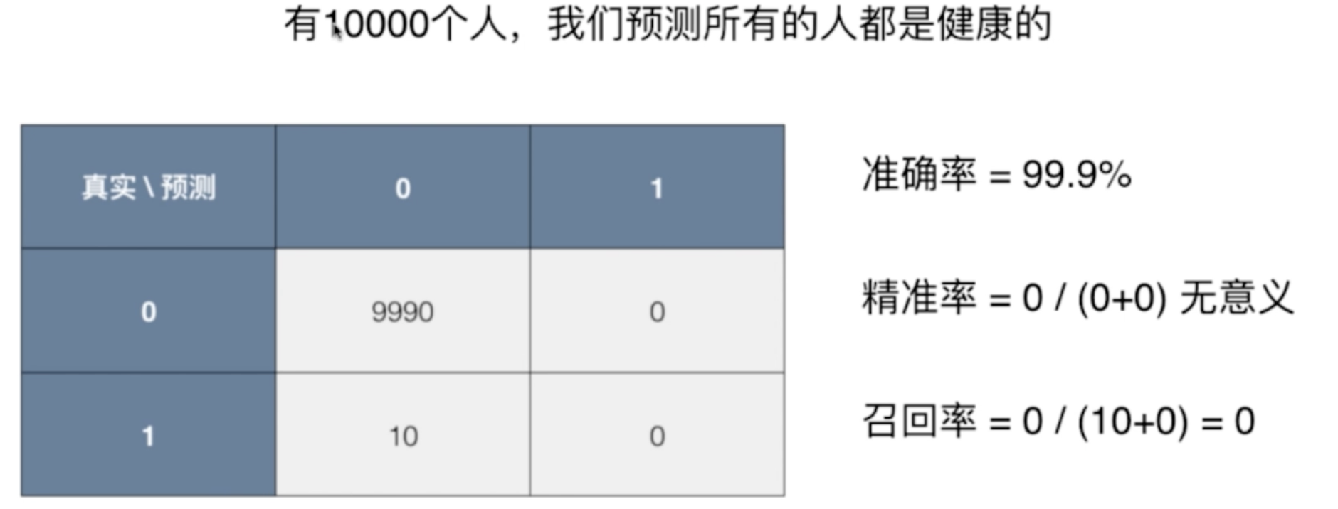
如果患病率为 0.1%，我们的系统预测所有人都是健康，即可达到99.9%的准确率。
如果患病率为0.01%，我们的系统预测所有人都是健康，可达到99.99%的准确率

结论：对于极度偏斜(Skewed Data)的数据，只使用分类准确度是远远不够的。

解决方法：使用混淆矩阵做进一 步的分析

---

混淆矩阵 Confusion Matrix

对于二分类问题

• 行代表真实值
• 列代表预测值
  • 0 Negative
  • 1 Positive

	0	1
0	TN	FP
1	FN	TP

• TN: True Negative，预测 negative 正确
• FP: False Positve，预测 postive 错误
• FN: False Negative，预测 negative 错误
• TP: True Positve，预测 postive 正确

---

精准率和召回率

	0	1
0	TN 9978	FP 12
1	FN 2	TP 8

---

精准率

预测数据中，遇到到100个数据为1，实际有多少个1。

$ precision = \frac{ TP }{ TP + FP } $

上述数据中 精准率 = 8/(12+8) = 40%

---

什么时候注重精准率？
如：股票预测。

---

召回率

预测数据中，有一百个为1的数据，预测到了多少个1。

$ recall = \frac{ TP }{ TP + FN } $

上述数据中 召回率 = 8/(2+8) = 80%

---

什么时候注重召回率率？
如：疾病诊断。

这个时候，准确率低一点没关系。可以进一步确诊。

---

为什么好？

精准率和召回率 为什么 比分类准确度好？

以下案例使用精准率没有意义。

---

F1 Score

F1 会兼顾 精准率 和 召回率，是两者的调和平均值（而非算数平均值）。

F 1 = 2 ∗ p r e s i c i o n ∗ r e c a l l p r e s i c i o n + r e c a l l F1 = \frac{ 2 * presicion * recall }{ presicion + recall } F1=presicion+recall2∗presicion∗recall​

1 F 1 = 1 2 ( 1 p r e c i s i o n + 1 r e c a l l ) \frac{1}{F1} = \frac{1}{2} ( \frac{1}{ precision } + \frac{1}{ recall } ) F11​=21​(precision1​+recall1​)

为什么取调和平均值？
调和平均值有个特点：如果两者极度不平衡，比如某一个特别高，一个特别低，那么F1也会很低。

当 recall 和 precision 都为1时，F1 取最大值 1；
当两者都为 0 时，F1 为 0。

---

代码实现

F1 的代码实现

import numpy as np
 
def f1_score(precision, recall):
    try:
        return 2 * precision * recall / (precision + recall)
    except:
        return 0.0
 
# 如果两者相等，则 f1 的值也等于他们
precision = 0.5
recall = 0.5
f1_score(precision, recall)
# 0.5
 
# 如果两个不同，结果会被拉低
precision = 0.1
recall = 0.9
f1_score(precision, recall)
# 0.18000000000000002
 
# 有一个为0，就会为0
precision = 0.0
recall = 1.0
f1_score(precision, recall)
# 0.0

---

引入真实数据

from sklearn import datasets

digits = datasets.load_digits()
X = digits.data
y = digits.target.copy()

y[digits.target==9] = 1
y[digits.target!=9] = 0

 

---

混淆矩阵，精准率、召回率的实现

def TN(y_true, y_predict):
    assert len(y_true) == len(y_predict)
    return np.sum((y_true == 0) & (y_predict == 0))

def FP(y_true, y_predict):
    assert len(y_true) == len(y_predict)
    return np.sum((y_true == 0) & (y_predict == 1))

def FN(y_true, y_predict):
    assert len(y_true) == len(y_predict)
    return np.sum((y_true == 1) & (y_predict == 0))
    
def TP(y_true, y_predict):
    assert len(y_true) == len(y_predict)
    return np.sum((y_true == 1) & (y_predict == 1))

def confusion_matrix(y_true, y_predict):
    return np.array([
        [TN(y_true, y_predict), FP(y_true, y_predict)],
        [FN(y_true, y_predict), TP(y_true, y_predict)]
    ])

 
def precision_score(y_true, y_predict):
    tp = TP(y_true, y_predict)
    fp = FP(y_true, y_predict)
    try:
        return tp / (tp + fp)
    except:
        return 0.0
        
def recall_score(y_true, y_predict):
    tp = TP(y_true, y_predict)
    fn = FN(y_true, y_predict)
    try:
        return tp / (tp + fn)
    except:
        return 0.0
    
y_log_predict = log_reg.predict(X_test)

TN(y_test, y_log_predict)		# 403
FP(y_test, y_log_predict)		# 2
FN(y_test, y_log_predict)		# 9  
TP(y_test, y_log_predict)		# 36

confusion_matrix(y_test, y_log_predict)
'''
array([[403,   2],
           [  9,  36]])
'''

precision_score(y_test, y_log_predict)	# 0.94736842105263153 

recall_score(y_test, y_log_predict)   # 0.80000000000000004

---

scikit-learn中的混淆矩阵，精准率、召回率、F1

from sklearn.model_selection import train_test_split

X_train, X_test, y_train, y_test = train_test_split(X, y, random_state=666)
 
from sklearn.linear_model import LogisticRegression

log_reg = LogisticRegression()
log_reg.fit(X_train, y_train)
log_reg.score(X_test, y_test)
# 0.97555555555555551
 
y_predict = log_reg.predict(X_test)
 
from sklearn.metrics import confusion_matrix, precision_score, recall_score, f1_score

confusion_matrix(y_test, y_predict)  # 混淆矩阵
'''
    array([[403,   2],
           [  9,  36]])
'''
 precision_score(y_test, y_predict)
# 0.94736842105263153
 
recall_score(y_test, y_predict)
# 0.80000000000000004
 
f1_score(y_test, y_predict)
# 0.86746987951807231

---

Precision-Recall 的平衡

阈值对精准率和召回率的影响

上图 星星 为1；
可以看出，随着阈值增大，精准率变高，召回率变低；
Precision 和 Recall 是互相矛盾的指标，无法同时很大。

通俗理解，想要精准率高，就是要特别有把握的数据才去标记；但这样就会漏掉很多真实为1的样本。

---

代码实现阈值的调整

# decision_function 做决策的函数，可以知道每个对应的 score 值是多少  
  
log_reg.decision_function(X_test)[:10]
# array([-22.05700185, -33.02943631, -16.21335414, -80.37912074, -48.25121102, -24.54004847, -44.39161228, -25.0429358 ,  -0.97827574, -19.71740779])
 
log_reg.predict(X_test)[:10]
# array([0, 0, 0, 0, 0, 0, 0, 0, 0, 0])

 
decision_scores = log_reg.decision_function(X_test)
 
np.min(decision_scores)
# -85.686124167491727
 
np.max(decision_scores)
# 19.889606885682948

---

阈值使用 5

y_predict_2 = np.array(decision_scores >= 5, dtype='int')
 
confusion_matrix(y_test, y_predict_2) # array([[404,   1], [ 21,  24]])

 
precision_score(y_test, y_predict_2)	# 0.95999999999999996
 
recall_score(y_test, y_predict_2)  # 0.53333333333333333

---

阈值使用 -5

y_predict_3 = np.array(decision_scores >= -5, dtype='int')
 
confusion_matrix(y_test, y_predict_3)
# array([[390,  15], [  5,  40]])

 
precision_score(y_test, y_predict_3) # 0.72727272727272729
 
recall_score(y_test, y_predict_3)  #0.88888888888888884

---

阈值如何选取 – PR 曲线

from sklearn.metrics import precision_score
from sklearn.metrics import recall_score

precisions = []
recalls = []

thresholds = np.arange(np.min(decision_scores), np.max(decision_scores), 0.1)

for threshold in thresholds:
    y_predict = np.array(decision_scores >= threshold, dtype='int')
    precisions.append(precision_score(y_test, y_predict))
    recalls.append(recall_score(y_test, y_predict))


plt.plot(thresholds, precisions)
plt.plot(thresholds, recalls)
plt.show()

---

Precision-Recall 曲线

# x 轴为精确率，recall 为召回率；两者的关系
plt.plot(precisions, recalls)
plt.show()

---

scikit-learn中的Precision-Recall曲线

from sklearn.metrics import precision_recall_curve

precisions, recalls, thresholds = precision_recall_curve(y_test, decision_scores) 
 
# 为什么是145？上述函数会自动根据数据取最适合的步长
precisions.shape	# (145,)  
recalls.shape # (145,)
thresholds.shape  # (144,)
 
plt.plot(thresholds, precisions[:-1])
plt.plot(thresholds, recalls[:-1])
plt.show()

---

plt.plot(precisions, recalls)
plt.show()

---

PR 曲线中急剧下降的点，很有可能就是 precision 和 recall 达到平衡的点。

---

外面曲线对应的模型，优于里面曲线对应的模型；
里面的描述比较抽象，也可以使用曲线包的面积来描述。

---

ROC 曲线

ROC ：Receiver Operation Characteristic Curve
常用语统计学，描述TPR和FPR之间的关系。

---

TPR 就是召回率，预测为1 占总为1 的比例
T P R = T P T P + F N TPR = \frac{ TP }{ TP + FN } TPR=TP+FNTP​

FPR: False Position Rate，预测为0 占总为0的比例
F P R = F P T N + F P FPR = \frac{ FP }{ TN + FP } FPR=TN+FPFP​

可以发现，随着阈值降低， TPR 和 FPR 都变大；这两者变化趋势一致；

---

TPR & FPR 代码实现

def TPR(y_true, y_predict):
    tp = TP(y_true, y_predict)
    fn = FN(y_true, y_predict)
    try:
        return tp / (tp + fn)
    except:
        return 0.


def FPR(y_true, y_predict):
    fp = FP(y_true, y_predict)
    tn = TN(y_true, y_predict)
    try:
        return fp / (fp + tn)
    except:
        return 0.
    

---

ROC 的代码实现

from playML.metrics import FPR, TPR

fprs = []
tprs = []
thresholds = np.arange(np.min(decision_scores), np.max(decision_scores), 0.1)

for threshold in thresholds:
    y_predict = np.array(decision_scores >= threshold, dtype='int')
    fprs.append(FPR(y_test, y_predict))
    tprs.append(TPR(y_test, y_predict))
 

plt.plot(fprs, tprs)
plt.show()

---

scikit-learn中的ROC

from sklearn.metrics import roc_curve

fprs, tprs, thresholds = roc_curve(y_test, decision_scores)
 
plt.plot(fprs, tprs)
plt.show()

---

ROC AUC

AUC：area under curve

from sklearn.metrics import roc_auc_score

# 计算面积
roc_auc_score(y_test, decision_scores)  # 0.98304526748971188

roc 面积更大的模型，被认为是更佳的模型。

---

混淆矩阵的实现

import matplotlib.pyplot as plt
import itertools

def plot_confusion_matrix(cm, classes,
                          title='Confusion matrix',
                          cmap=plt.cm.Blues):
    """
    This function prints and plots the confusion matrix.
    """
    plt.imshow(cm, interpolation='nearest', cmap=cmap)
    plt.title(title)
    plt.colorbar()
    tick_marks = np.arange(len(classes))
    plt.xticks(tick_marks, classes, rotation=0)
    plt.yticks(tick_marks, classes)

    thresh = cm.max() / 2.
    for i, j in itertools.product(range(cm.shape[0]), range(cm.shape[1])):
        plt.text(j, i, cm[i, j],
                 horizontalalignment="center",
                 color="white" if cm[i, j] > thresh else "black")

    plt.tight_layout()
    plt.ylabel('True label')
    plt.xlabel('Predicted label')

---

调用

from sklearn.metrics import confusion_matrix

LR_model = LogisticRegression()
LR_model = LR_model.fit(X_train, y_train)
y_pred = LR_model.predict(X_test)
cnf_matrix = confusion_matrix(y_test,y_pred)

# 召回率
print("Recall metric in the testing dataset: ", cnf_matrix[1,1]/(cnf_matrix[1,0] + cnf_matrix[1,1]))

# 精度
print("accuracy metric in the testing dataset: ", (cnf_matrix[1,1] + cnf_matrix[0,0])/(cnf_matrix[0,0] + cnf_matrix[1,1]+cnf_matrix[1,0]+cnf_matrix[0,1]))

# Plot non-normalized confusion matrix
class_names = [0,1]
plt.figure()
plot_confusion_matrix(cnf_matrix, classes=class_names, title='Confusion matrix')
plt.show()

---

---

---

标签：plt,predict,ML,算法,score,recall,test,评价,true
来源： https://blog.csdn.net/lovechris00/article/details/122281390

本站声明： 1. iCode9 技术分享网（下文简称本站）提供的所有内容，仅供技术学习、探讨和分享；
2. 关于本站的所有留言、评论、转载及引用，纯属内容发起人的个人观点，与本站观点和立场无关；
3. 关于本站的所有言论和文字，纯属内容发起人的个人观点，与本站观点和立场无关；
4. 本站文章均是网友提供，不完全保证技术分享内容的完整性、准确性、时效性、风险性和版权归属；如您发现该文章侵犯了您的权益，可联系我们第一时间进行删除；
5. 本站为非盈利性的个人网站，所有内容不会用来进行牟利，也不会利用任何形式的广告来间接获益，纯粹是为了广大技术爱好者提供技术内容和技术思想的分享性交流网站。